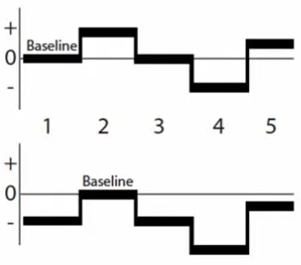
An event-related potential (ERP) is the electrical brain activity time-locked to an event (e.g. a stimulus, a response or a decision), obtained by averaging EEG segments (epochs) recorded around many repetitions of the event. An event-related field (ERF) is its MEG equivalent (the averaged magnetic field).
ERPs are used to study the timing of sensory, motor and cognitive processes (e.g. perception, attention, memory, language, error monitoring) with millisecond resolution, and clinically (e.g. evoked potentials in the diagnosis of sensory pathways).
The Averaging Model
A single EEG epoch contains the ERP and much larger ongoing activity and noise (often 20–50 μV), while the ERP components are a few microvolts. The classical ERP model assumes that each epoch is the sum of:
the ERP: identical in every epoch (the same waveform at the same latency, time-locked to the event)
the noise: the ongoing EEG and artifacts, random, with zero mean and unrelated to the event
Averaging \(N\) epochs keeps the ERP and reduces the noise: the standard deviation of the noise in the average decreases with \(\sqrt{N}\):
For example, with a noise of 20 μV, the residual noise is 2 μV after 100 epochs and 1.4 μV after 200 epochs; to halve the residual noise of 100 epochs, 400 epochs are needed. The number of epochs is a trade-off between the signal-to-noise ratio and the duration of the experiment (and the fatigue and habituation of the subject).
A simulated ERP: three components (P1 at 100 ms, N1 at 170 ms, P3 at 350 ms) modelled as Gaussian waves, sampled at 500 Hz from −200 to 800 ms:
The residual noise of the average (the standard deviation of the average minus the true ERP) follows \(\sigma / \sqrt{N}\):
ns = [1, 2, 5, 10, 20, 50, 100, 200, 400]residual = [std(vec(mean(epochs[:, 1:n]; dims =2)) .- erp_true) for n in ns]fig, ax =scatter(ns, residual; label ="residual noise of the average", figure = (size = fig_size,), axis = (ax_style..., xticks = [1, 10, 100, 400], xminorticksvisible =false, xscale = log10, yscale = log10, xlabel ="Number of epochs", ylabel ="Noise [μV]"))lines!(ax, ns, 15./sqrt.(ns); color =:red, label ="15 μV / √N")axislegend(ax; position =:rt)fig
Signal-to-noise ratio (SNR) of an ERP is often estimated as the peak (or mean) amplitude of the component divided by the standard deviation of the baseline (pre-stimulus) interval of the average.
Violations of the Model
The averaging model is a simplification:
Latency jitter: if a component occurs at a slightly different latency in each epoch, averaging smears it: the averaged component is lower and wider than in the single epochs. Components related to decisions (e.g. P3) vary with the reaction time and are particularly affected. Response-locked averaging or single-trial methods may be used instead.
Non-stationarity: the ERP changes during the experiment (habituation, learning, fatigue).
Event-related changes of the ongoing activity: the event can reset the phase of ongoing oscillations or change their power (event-related synchronization/desynchronization); oscillations that are not phase-locked to the event cancel out in the average and require time-frequency analysis.
The same P3 with a latency jitter (standard deviation 50 ms) between epochs:
p3_epochs =hcat([gauss(t, 8, 0.35+0.05*randn(), 0.060) for _ in1:n_ep]...)fig, ax =lines(t, gauss(t, 8, 0.35, 0.060); color =:black, label ="P3 without jitter", figure = (size = fig_size,), axis = (ax_style..., xlabel ="Time [s]", ylabel ="Amplitude [μV]"))lines!(ax, t, vec(mean(p3_epochs; dims =2)); color =:red, label ="average of jittered P3")axislegend(ax; position =:lt)fig
The area under the curve is preserved, but the peak amplitude is reduced: peak amplitudes underestimate components with variable latency, while mean amplitudes over a wide window are less affected.
Baseline Correction
The epochs contain slow drifts and offsets that are unrelated to the event. Baseline correction subtracts the mean of a pre-stimulus interval (the baseline, typically −200 to 0 ms) from every sample of the epoch (or of the average), separately for each channel, so that the ERP amplitudes are measured relative to the pre-stimulus activity:
Five epochs with random offsets (standard deviation 20 μV; with less noise than above, 3 μV, so that the offsets are visible) before and after baseline correction:
The baseline must not contain activity related to the event (e.g. anticipation, or the response to a preceding stimulus when the stimuli follow each other quickly); a difference between conditions already in the baseline is transferred (with the opposite sign) to the whole ERP.
Longer baselines give a more stable estimate of the offset (less affected by noise).
High-pass filtering removes slow drifts as well, but strong high-pass filters (> 0.1–0.5 Hz) distort slow ERP components.
Effects of choosing a baseline window:
In the frequency domain (time-frequency analysis), the baseline power is used to normalize the event-related power (e.g. as a change in dB or percent relative to the baseline).
In NeuroAnalyzer, average_epochs(obj; bl = (-0.2, 0)) averages the epochs and subtracts the baseline; see Event-Related Potentials.
ERP Components
An ERP component is a part of the waveform that reflects a specific neural process. Components are named by their polarity (P: positive, N: negative) and either their latency in milliseconds (N170, P300) or their order (P1, N1, P2, N2, P3); some have functional names (mismatch negativity, error-related negativity).
Component
Latency
Typical scalp distribution
Elicited by / reflects
P1
80–130 ms
occipital
visual stimuli; early sensory processing, modulated by attention
auditory deviants in a sequence of standards, even without attention
N2
200–350 ms
fronto-central
conflict, inhibition, novelty
P3a
250–350 ms
fronto-central
novel, unexpected stimuli (orienting)
P3b (P300)
300–600 ms
centro-parietal
task-relevant rare targets (oddball paradigm); its latency increases with the difficulty of the stimulus evaluation
N400
300–500 ms
centro-parietal
semantic incongruence (e.g. an unexpected word in a sentence)
P600
500–900 ms
centro-parietal
syntactic violations, reanalysis
ERN (error-related negativity)
0–100 ms after the response
fronto-central
errors (response-locked)
CNV (contingent negative variation)
between a warning and an imperative stimulus
fronto-central
anticipation, motor preparation
LRP (lateralized readiness potential)
before the response
central (C3/C4)
preparation of a hand movement
Latencies and distributions depend on the stimulus, the task and the subject (age, clinical group).
Stimulus-locked ERPs are averaged relative to the stimulus onset; response-locked ERPs relative to the response (e.g. the button press), which is better for components related to the response (ERN, LRP).
Measuring ERPs
Common measures of a component (in a predefined time window and channel or region of interest):
peak amplitude and peak latency: the maximum (or minimum) in the window; simple, but sensitive to noise (in noisy data the peak is biased towards larger values) and to latency jitter
mean amplitude: the mean voltage in the window; robust to noise and jitter, the most commonly recommended measure
area under the curve (and the fractional area latency: the time at which e.g. 50% of the area is reached)
difference waves: the difference between two conditions (e.g. target − standard), which isolates the processes that differ between them
Peak and mean P3 amplitude (300–400 ms) in averages of 20 epochs; the peak amplitude is systematically overestimated by the noise:
The time windows and channels must be chosen before looking at the data (e.g. from previous studies or from the average of all conditions), otherwise the results are biased (the “double dipping” problem).
Reverse Inference
ERP studies infer cognitive processes from components:
forward inference: a manipulation of a cognitive process (e.g. attention) changes a component (e.g. the N1 amplitude)
reverse inference: the presence or change of a component is used to infer that a process took place (e.g. “the N170 was larger, so the stimulus was processed as a face”)
Reverse inference is only as valid as the specificity of the component: if a component is elicited by several processes (e.g. the N170 is also elicited by words and by objects of expertise), its presence does not prove a particular process. It is strengthened by converging evidence (other components, behaviour, other methods).
ERFs
ERFs are obtained from MEG in the same way as ERPs from EEG. Their components correspond to the ERP components (often named with an “m” suffix, e.g. N1m, M100), but the magnetic fields are generated mainly by tangential sources (in the walls of the sulci) and are less distorted by the skull, which makes their sources easier to localize.
For the analysis of ERPs and ERFs in NeuroAnalyzer (epoching, averaging, baseline correction, plotting, peaks and topographic maps), see Event-Related Potentials.