usingNeuroAnalyzerusingStatisticsNeuroAnalyzer.progress_bar =falseeeg =import_edf("files/eeg/eeg.edf")# filtered 0.5-35 Hz (removes the DC offsets and the line noise of the raw# recording)NeuroAnalyzer.filter!(eeg; ch ="all", fprototype =:butterworth, ftype =:hp, cutoff =0.5, order =4)NeuroAnalyzer.filter!(eeg; ch ="all", fprototype =:fir, ftype =:lp, cutoff =35, bw =10)load_locs!(eeg; file_name ="files/locs/standard-10-20-cap19-elmiko.locs")# 60-second segmenteeg =crop(eeg; seg = (100, 160))
An EEG channel is always the voltage difference between two points: an electrode and a reference. The set of channels used to display or analyze the recording is a montage: e.g. all electrodes against one common reference (referential montage), or chains of neighboring electrode pairs (bipolar montage). Re-referencing computes a new montage from the recorded signals.
There Is No Reference-Free EEG
EEG amplifiers measure voltage differences; the absolute potential of a single electrode cannot be measured. Every electrode, including the reference, picks up brain and other body signals by volume conduction, so no point of the body is truly “silent”. The recorded signal of electrode \(i\) is
\[
V_i^{rec} = \phi_i - \phi_{ref}
\]
where \(\phi\) is the (unknown) potential. Changing to another common reference subtracts the same signal from all channels:
waveforms, amplitudes, spectra and connectivity depend on the reference: the same brain activity looks different with different references,
differences between channels do not depend on the common reference: \(V_i - V_j = \phi_i - \phi_j\) for any common reference,
the shape of a topographic map (the spatial pattern at a time point) does not depend on the common reference: the whole map is shifted by the same value, like a landscape described relative to a different sea level.
This does not hold for bipolar and Laplacian montages, which are spatial filters: each channel gets a different reference.
The recording used here is stored as recorded (physical reference: the reference electrode of the amplifier, not recorded as a channel):
println(eeg.header.recording[:reference])
physical
Alpha band power (8-12 Hz) in the same signal with different references, and the difference between F3 and P3:
refs = ["recorded"=> eeg,"Cz"=>reference_ce(eeg; ch ="Cz"),"linked ears"=>reference_a(eeg; type =:l),"average"=>reference_avg(eeg),"Laplacian"=>reference_plap(eeg)]
println(rpad("reference", 13), rpad("alpha power [μV²]", 32), "SD(F3 - P3)")println(rpad("", 13), "Fz Cz O1 T3")for (name, obj) in refs# labels of the re-referenced channels get a suffix, e.g. "Fz-avg" ch =labels(obj)[get_channel(obj; ch ="eeg")] bp =vec(band_power(obj; ch ="eeg", flim = (8, 12)))idx(l) =findfirst(x -> x == l ||startswith(x, l *"-"), ch) f3p3 = obj.data[get_channel(obj; ch = ch[idx("F3")]), :, 1] .- obj.data[get_channel(obj; ch = ch[idx("P3")]), :, 1]println(rpad(name, 13),join([rpad(round(bp[idx(l)]; digits =1), 7) for l in ["Fz", "Cz", "O1", "T3"]])," ", round(std(f3p3); digits =2))end
The power at each electrode depends on the reference: with the Cz reference, Cz itself is flat (power 0), and in the recorded signal Fz has almost no alpha activity, probably because the reference electrode of the amplifier was close to it. The difference F3 - P3 is the same for all common references (recorded, Cz, linked ears, average), but not for the Laplacian.
The topographic maps of the same time point (a large wave visible in all channels at 103.9 s), scaled to [-1, 1]: the maps for linked ears and the average reference are identical (as is the map of the recorded signal), the Laplacian map is different:
one electrode (e.g. Cz) or the mean of a few (A1, A2)
widespread activity
activity and artifacts of the reference are in all channels
average reference
the mean of all electrodes
widespread activity
needs many, evenly distributed, clean channels
Laplacian
the (weighted) mean of the nearest neighbors
local activity
removes widespread activity; edge electrodes
bipolar
the neighboring electrode in a chain
local activity, gradients
removes activity common to both electrodes
Montages as spatial filters
Bipolar and Laplacian montages are spatial high-pass filters: activity common to neighboring electrodes (widespread rhythms, distant sources, common artifacts) is removed, local activity is enhanced. Common and average references keep the widespread activity.
Common Electrode Reference
All channels are referenced to one electrode or to the mean of several electrodes. Typical choices:
Reference
Use
Notes
vertex (Cz)
recording reference of many systems
Cz is close to many sources; central channels have low amplitude
ears (A1, A2)
clinical EEG
close to the temporal lobes (temporal activity is reduced); ECG artifacts, often larger on the left
mastoids (M1, M2)
ERP research
as ears; poor contact of a single mastoid electrode contaminates all channels
nose, Fpz
some research systems
eye movement artifacts
reference_ce() references the EEG channels to one channel or to the mean (or median, med = true) of several channels:
["Fp1-Cz", "Fp2-Cz", "F3-Cz", "F4-Cz"]
common (Fp1, Fp2 averaged)
The labels of the re-referenced channels get a suffix with the reference, and the reference is stored in the header. Only EEG channels are re-referenced (EOG, ECG and the reference channels A1, A2 are not changed). With a single reference electrode that is an EEG channel, this channel becomes flat.
Ears and mastoids
reference_a() (auricular electrodes A1, A2) and reference_m() (mastoid electrodes M1, M2) use the two electrodes in three ways (type):
:l (default): linked - the mean of both electrodes, for all channels,
:i: ipsilateral - A1 (M1) for the channels over the left hemisphere, A2 (M2) for the right,
:c: contralateral - A2 (M2) for the left channels, A1 (M1) for the right.
With :i and :c, the midline channels (Fz, Cz, Pz) use the linked reference:
This recording has no mastoid electrodes; to show reference_m(), the ear electrodes are renamed:
eeg_m =rename_channel(eeg; ch ="A1", name ="M1")rename_channel!(eeg_m; ch ="A2", name ="M2")eeg_mc =reference_m(eeg_m; type=:c)
Tip: “Linked” ears or mastoids should be computed (as here), not wired together during the recording: physically linked electrodes form a low-resistance path that distorts the scalp potentials.
Average Reference
The common average reference (CAR) subtracts the mean of all EEG channels from each channel. It is based on the fact that the potentials over a closed surface surrounding all sources sum to zero; the mean of the electrodes then approximates zero potential. The approximation is good only with many electrodes covering the head evenly (64 or more, including the lower parts of the head); with 19 electrodes of the 10-20 system it is rough.
After average referencing, the channels sum to zero at each time point:
Fp1, Fp2 (eye blinks) and O1, O2 (head movements) are not used to compute the reference
exclude_current = true
each channel is excluded from its own reference
med = true
median instead of mean: less sensitive to single noisy channels
weighted = true
channels weighted by inverse distance (requires channel locations): close channels count more
eeg_avg2 =reference_avg(eeg; exclude_fpo =true, med =true)
Advantages: no single reference electrode dominates; the reference is not attached to one region of the head; recommended for high-density recordings and for source analysis.
where \(S_i\) are the neighbors of electrode \(i\) and \(d_{ij}\) the distances (for the unweighted Laplacian, \(g_{ij} = 1/|S_i|\)). The result approximates the second spatial derivative of the scalp potential, which is related to the current flowing through the skull at the electrode (current source density). It enhances activity generated directly under the electrode and removes widespread activity and volume-conducted activity from distant sources; it does not depend on the recording reference.
Small Laplacian uses the nearest neighbors, large Laplacian the next-nearest neighbors (at a larger distance), which is less sensitive to noise and to small sources:
NeuroAnalyzer computes the nearest-neighbor Laplacian in two ways (both require channel locations):
reference_plap(): planar - neighbors and distances in the 2-D projection of the electrode positions (as in topographic maps),
reference_slap(): spherical - great-circle distances on the sphere, which accounts for the curvature of the head.
nn is the number of neighbors (default 4), weighted = true weights them by inverse distance, and med = true uses the (weighted) median:
eeg_plap =reference_plap(eeg; nn =4)eeg_wplap =reference_plap(eeg; nn =6, weighted =true)eeg_slap =reference_slap(eeg; nn =4, weighted =true)
println(eeg_wplap.header.recording[:reference])
weighted planar Laplacian (6)
Tip: Electrodes at the edge of the montage (e.g. Fp1, T3, O2) do not have neighbors on all sides, so their Laplacian is less accurate. The spline-based surface Laplacian (current source density, below), which uses all electrodes, is more accurate but requires a dense montage.
Current Source Density (CSD)
The current source density (CSD) is the surface Laplacian of the scalp potential, computed with spherical splines (Perrin et al. 1989): a smooth function on a sphere is fitted to the potentials of all electrodes, and its second spatial derivative is calculated analytically at each electrode. It is proportional to the current flowing radially through the skull into (sink) or out of (source) the scalp at the electrode. Compared with the nearest-neighbor Laplacian, it uses all electrodes and the curvature of the head, and is more accurate, especially at the edge of the montage.
Like the Laplacian, CSD:
is reference-free: the Laplacian of a constant (a change of the reference adds the same value to all channels) is zero,
enhances local activity (sources close to the electrode) and removes widespread, volume-conducted activity: it sharpens topographic maps,
needs channel locations and a sufficient number of electrodes (≥ 32 is recommended; with 19 electrodes it is a rough estimate).
csd() transforms the EEG channels (channel type and data type "csd"):
eeg_csd =csd(eeg)
The result does not depend on the reference of the data:
stiffness of the spline (2-10): higher values give a smoother surface
n
8
number of Legendre polynomial terms
lambda
1e-5
regularization: larger values smooth the fit (less sensitive to noise of single channels)
The second derivative amplifies noise and small differences between neighboring channels; stiffer splines and more regularization give smoother (and smaller) CSD:
for (m, l) in [(3, 1e-5), (4, 1e-5), (5, 1e-5), (4, 1e-3)] x =csd(eeg; m = m, lambda = l).data[ch_csd, :, :]println("m = ", m, ", lambda = ", l, ": SD ", round(std(x); digits =1))end
m = 3, lambda = 1.0e-5: SD 97.7
m = 4, lambda = 1.0e-5: SD 61.6
m = 5, lambda = 1.0e-5: SD 33.9
m = 4, lambda = 0.001: SD 19.7
Tip: The electrode positions are projected onto a sphere of radius 1, so the values (labeled μV/m²) correspond to a head of radius 1 m, as in MNE with sphere = (0, 0, 0, 1); they are proportional to the true current density, and their scale depends on m and lambda. Compare CSD values only between data computed with the same parameters.
CSD is used e.g. to separate overlapping ERP components and their generators (Kayser and Tenke 2006) and before connectivity analyses, where it reduces spurious connectivity caused by volume conduction.
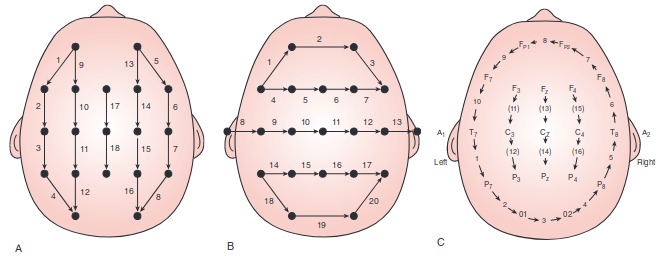
Bipolar Montages
In a bipolar montage, each channel is the difference between two neighboring electrodes, usually arranged in chains:
longitudinal (A, “double banana”): chains from front to back, e.g. Fp1-F7, F7-T3, T3-T5, T5-O1,
transverse (B): chains from left to right, e.g. F7-F3, F3-Fz, Fz-F4, F4-F8,
circumferential (C): a closed loop around the head (with the central chains inside).
Common chains of the longitudinal montage (10-20 system):
Chain
Channels
left temporal
Fp1-F7, F7-T3, T3-T5, T5-O1
left parasagittal
Fp1-F3, F3-C3, C3-P3, P3-O1
central
Fz-Cz, Cz-Pz
right parasagittal
Fp2-F4, F4-C4, C4-P4, P4-O2
right temporal
Fp2-F8, F8-T4, T4-T6, T6-O2
Bipolar montages are standard in clinical EEG: they enhance local activity, cancel activity and artifacts common to neighboring electrodes, and localize focal activity by phase reversal.
Phase reversal
The electrode closest to a focal source has the most extreme potential. In a chain, it is the second electrode of one channel and the first electrode of the next, so the two channels have opposite signs. A negative focus at T4, with the potentials:
Electrode
Fp2
F8
T4
T6
O2
μV
-5
-20
-40
-10
0
gives the channels of the right temporal chain:
Channel
Value
Fp2-F8
-5 - (-20) = +15 μV
F8-T4
-20 - (-40) = +20 μV
T4-T6
-40 - (-10) = -30 μV
T6-O2
-10 - 0 = -10 μV
The sign changes between F8-T4 and T4-T6: the source is at their common electrode, T4. In the clinical display convention (negative up), the deflections of F8-T4 and T4-T6 point towards each other (negative phase reversal).
In a referential montage, there is no phase reversal: the focus is the electrode with the largest amplitude (provided the reference is not close to the source).
End of chain
If the source is at the first or last electrode of a chain (e.g. Fp2 or O2), there is no channel on the other side and no phase reversal. A circumferential montage, which has no ends, or a referential montage, helps in such cases.
Bipolar montages in NeuroAnalyzer
reference_custom() creates any montage from a list of channels ("Fz") and channel pairs ("Fz-Cz" = Fz − Cz); by default, it creates the longitudinal bipolar montage:
All EEG channels are replaced by the montage channels; other channels (here A1, A2, EOG, ECG) are kept. A montage channel is marked as bad if one of its electrodes is marked as bad.
Locations of montage channels
A single channel (e.g. "Fz") keeps its location. The location of a channel pair is set by the loc option:
loc = :mid (default): the midpoint between the two electrodes. A bipolar channel measures the potential difference between both electrodes, so it reflects activity at and between them. The midpoint of the Cartesian coordinates is projected back onto the head surface, and the spherical coordinates are recalculated from it; the polar coordinates are the midpoint between the two electrodes on the topographic plot.
loc = :first: the location of the first electrode of the pair (as in MNE). This moves each channel half the inter-electrode distance towards the beginning of its chain.
plot_locs(eeg_bip, ch ="eeg", gui =false)
eeg_bip_first =reference_custom(eeg; loc =:first)
Note: A bipolar channel measures the potential gradient along one direction, not the potential at a point. Topographic maps of bipolar montages are therefore only approximate and should not be interpreted as maps of referential data.
The right temporal chain; signal plots use the clinical convention (negative up):
The labels in the list must match the channel labels of the recording (e.g. T3/T4/T5/T6 in the old 10-20 nomenclature, T7/T8/P7/P8 in the 10-10 nomenclature).
Montage files
Montages can be stored in text files: the first line is the name of the montage, each next line one channel or channel pair; empty lines and lines starting with # are ignored. Example files are in the montages/ folder of NeuroAnalyzer:
edit_montage() opens a montage file in the text editor of the system (on Linux: the editor set in the EDITOR environment variable):
edit_montage("my_montage.mnt")
Choosing a Reference
Purpose
Recommended
Notes
focal activity (spikes, local sources)
bipolar, Laplacian
phase reversal (bipolar); local activity enhanced
widespread activity (generalized discharges)
common electrode (ears, mastoids), average
bipolar and Laplacian montages cancel it
ERPs
average (dense montages), linked mastoids
follow the convention of the field, so that results can be compared
hemispheric asymmetry
average, linked ears/mastoids
an ipsilateral or one-sided reference creates spurious asymmetry
finding bad electrodes
referential and bipolar montages
a bad electrode stands out in all channels that use it
source analysis, high-density EEG
average
the reference must be modelled; the average is standard
There is no “correct” reference: it should be chosen for the question asked, reported in publications, and, if possible, results should be checked with another reference.
Re-reference: an average reference must be computed only from clean channels.
Remove artifacts (e.g. ICA), split into epochs, reject bad epochs, analyze.
All referencing functions return a new object; their ! versions (reference_avg!(), reference_ce!(), …) modify the object in place. The reference is recorded in the header and in the processing history.